Solving Linear Programming Problems with Grey Data
Michael Gr. Voskoglou1*
1Emeritus of Mathematical Sciences, Western Greece, Patras, Greece, School of Technological Applications Graduate Technological Educational Institute, Patras, Greece .
http://dx.doi.org/10.13005/OJPS03.01.04
A Grey Linear Programming problem differs from an ordinary one to the fact that the coefficients of its objective function and / or the technological coefficients and constants of its constraints are grey instead of real numbers. In this work a new method is developed for solving such kind of problems by the whitenization of the grey numbers involved and the solution of the obtained in this way ordinary Linear Programming problem with a standard method. The values of the decision variables in the optimal solution may then be converted to grey numbers to facilitate a vague expression of it, but this must be strictly checked to avoid non creditable such expressions. Examples are also presented to illustrate the applicability of our method in real life applications.
Copy the following to cite this article:
Voskoglou M. G. Solving Linear Programming Problems with Grey Data. Orient J Phys Sciences 2018;3(1).
DOI:http://dx.doi.org/10.13005/OJPS03.01.04Copy the following to cite this URL:
Voskoglou M. G. Solving Linear Programming Problems with Grey Data. Orient J Phys Sciences 2018;3(1). Available from: https://bit.ly/3oWpBJH
Download article (pdf) Citation Manager Publish History
Introduction
It is well known that Linear Programming (LP) is a technique for the optimization (maximization or minimization) of a linear objective function subject to linear equality and inequality constraints. The feasible region of a LP problem is a convex polytope, which is a generalization of the three-dimensional polyhedron in the n-dimensional space Rn, where R denotes the set of the real numbers and n is an integer, n>.2
In 1975 the Soviet Leonid Kantorovich and the Dutch-American T. C. Koopmans shared the Nobel prize in Economics for their work, at the end of the 1930’s, on formulating and solving LP problems. A LP algorithm determines a point of the LP polytope, where the objective function takes its optimal value, if such a point exists. In 1947 George B. Dantzic invented the SIMPLEX algorithm1 that for the first time efficiently tackled the LP problem in most cases. Note that earlier, in 1941, Frank Lamen Hitchcock gave a very similar to the SIMPLEX algorithm solution for the Transportation Problem. In 1948
Dantzic, adopting a conjecture of John von Neuman, who worked on an equivalent problem in Game Theory, provided a formal proof of the theory of Duality.2 According to the above theory every LP problem can be converted to a dual problem the optimal solution of which, if it exists, provides an optimal solution for the original problem. A large breakthrough in the field came also in 1984, when Narendra Karmakar introduced a new interior-point method for solving LP problems. For more details about the history of LP the reader my look at,3 while for general facts about the SIMPLEX algorithm we refer to Chapters 3 and 4 of.4
LP, apart from mathematics, is widely used nowadays in business and economics, in several engineering problems, etc. Many practical problems of Operations Research can be expressed as LP problems. However, in large and complex systems, like the socio-economic, the biological ones, etc. ., it is often very difficult to solve satisfactorily the LP problems with the standard theory, since the necessary data can not be easily determined precisely and therefore estimates of them are used in practice. The reason for this is that such kind of systems they usually involve many different and constantly changing factors the relationships among which are indeterminate, making their operation mechanisms not clear. In order to obtain good results in such cases one may apply either techniques of fuzzy logic (Fuzzy LP, e.g. see5-7, etc.) or of the grey systems theory (Grey LP, e.g. see,8,9 etc.).
In this work we develop a new technique for solving grey LP problems. The rest of the paper is formulated as follows: In the second Section the background information is recalled about the Grey Numbers (GNs) which is necessary for the understanding of the paper. In the third Section our method for solving grey LP problems is developed and examples are presented illustrating it. Finally, the fourth Section is devoted to our conclusions and some hints for future research on the subject.
Grey Numbers
An investigated object with “poor” information is referred to as a grey system. An effective tool for handling the approximate data of a grey system is the use of GNs. In an earlier work we have presented the GNs and their arithmetic and we have applied them for assessing the mean performance of a group of objects (students, players, etc.) participating in a certain activity.10 Therefore, here we shall recall only the information about GNs which is necessary for the understanding of the present work.
A GN is an indeterminate number whose probable range is known, but which has unknown position within its boundaries. Therefore, a GN, say A, can be expressed mathematically in the form
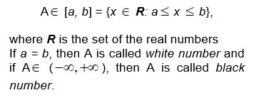
Let us denote by w(A) the white number with the highest probability to be the representative value of the GN A. E[a, b]. The technique of determining the value of w(A) is called whitenization of A.
One usually defines w(A) = (1- t)a + tb,
with t in.0,1 This is known as the equal weight whitenization. When the distribution
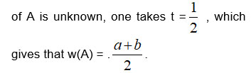
For general facts on GNs we refer to the book.11 Further, for the needs of the present paper we introduce the following definition:
The GN A [a, b] has Rank of Greyness (RoG) equal to x, with x in R, if, and only if
b - a = x. We write then RoG (A) = x. Therefore, for a white number A we have
RoG (A) =0, whereas the RoG of a black number is defined to be equal to + .
.
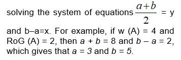
Note that, if the values w(A) = y and
RoG (A) = x are known, then the GN A [a, b] can be easily determined by
A Method of Solving Grey LP Problems
The general form of a Grey LP problem is the following:
Maximize (or minimize) the linear expression F = A1x1 + A2x2 +….+ Anxn subject to constraints of the form xj 0,
Ai1x1+ Ai2x2 +…..+ Ainxn <(>) Bi, where
i = 1, 2, …, m , j = 1, 2,,,, n and Aj, Aij, Bi are GNs.
The proposed in this work method for solving a Grey LP problem involves the following steps:
- Whitenization of the GNs Aj, Aij and Bi.
- Solution of the obtained by the previous step ordinary LP problem with the standard theory.
- Conversion of the values of the decision variables in the optimal solution to GNs with the desired RoG.
The last step is not compulsory, but it is useful in problems of fuzzy structure, where a vague expression of their solution is often preferable than the crisp one.
The following examples illustrate the applicability of our method: in real life applications:
Example 1: A furniture-making factory constructs tables and desks. It has been statistically estimated that the construction of a group of tables needs 2-3 working hours (w.h.) for assembling, 2.5-3.5 w.h. for elaboration (plane, etc.) and 0.75-1.25 w.h. for polishing. On the other hand, the construction of a group of desks needs 0.8-1.2, 2-4 and 1.5-2.5 w.h. for each of the above procedures respectively. According to the factory’s existing number of workers, no more than 20 w.h. per day can be spent for the assembling, no more than 30 w.h. for the elaboration and no more than 18 w.h. for the polishing of the tables and desks. If the profit from the sale of a group of tables is between 2.7 and 3.3 thousand euros and of a group of desks between 3.8 and 4.2 thousand euros,1 find how many groups of tables and desks should be constructed daily to maximize the factory’s total profit. Express the problem’s optimal solution with GNs of RoG equal to 1.
Solution: Let x1 and x2 be the groups of tables and desks to be constructed daily. Then the problem is mathematically formulated as follows:
Maximize F = [2.7, 3.3]x1 + [3.8, 4.2]x2 subject to constraints x1, x2 > 0 and
[2, 3]x1 + [0.8, 1.2]x2 <[20, 20]
[2.5, 3.5]x1 + [2, 4]x2 < [30, 30]
[0.75, 1.25]x1 + [1.5,2.5]x2 < [16, 16]
The whitenization of the GNs involved leads to the following LP maximization problem of canonical form:
Maximize f(x1, x2) = 3x1 + 4x2 subject to the constraints x1, x2 >0 and
2.5x1 + x2 <20
3x1 + 3x2 < 30
x1 + 2x2 <16
Adding the slack variables s1, s2, s3 for converting the last three inequalities to equations one forms the problem’s first SIMPLEX matrix, which corresponds to the feasible solution f(0, 0) = 0, as follows:
Denote by L1, L2, L3, L4 the rows of the above matrix, the fourth one being the net evaluation row. Since -4 is the smaller (negative) number of the net evaluation
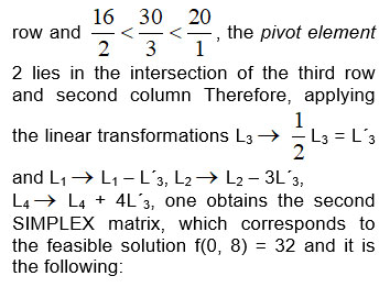
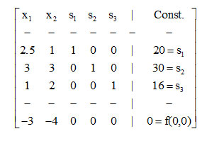
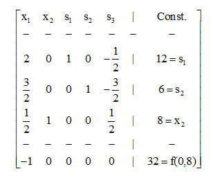
In this matrix the pivot element 3/2 lies in the intersection of the second row and first column, therefore working as above one obtains the third SIMPLEX matrix, which is:
Since there is no negative index in the net evaluation row, this is the last SIMPLEX matrix. Therefore f(4, 6) = 36 is the optimal solution maximizing the objective function. Further, since both the decision variables x1 and x2 are basic variables, i.e. they participate in the optimal solution, the above solution is unique.
Converting the values of the decision variables in the above solution to GNs with RoG equal to 1 one finds that
x1[3.5, 4.5] and x2[5.5, 6.5].
Therefore a vague expression of the solution states that the factory’s maximal profit corresponds to a daily production between 3.5 and 4.5 groups of tables and between 5.5 and 6.5 groups of desks.
However, considering for example the extreme values of the daily construction of 4.5 groups of tables and 6.5 groups of desks, one finds that it needs 33 in total w.h. for elaboration, whereas the maximum available w.h. are only 30. In other words, a vague expression of the solution does not guarantee that all the values of the decision variables within the boundaries of the corresponding GNs are feasible solutions.
Example 2: Three kinds of food, say T1, T2 and T3, are used in a poultry farm for feeding the chickens, their cost varying between 38 - 42, 17 - 23 and 55 - 65 cents per kilo respectively. The food T1 contains 1.5 - 2.5 units of iron and 4 - 6 units of vitamins per kilo, T2 contains 3.2 - 4.8, 0.6 – 1.4 and T3 contains 1.7 – 2.3, 0.8 – 1.2 units per kilo respectively. It has been decided that the chickens must receive at least 24 units of iron and 8 units of vitamins per day. How one must mix the three foods so that to minimize the cost of the food? Express the problem’s solution with GNs of RoG equal to 2.
Solution: Let x1, x2 and x3 be the quantities in kilos for each food to be mixed. Then, the problem’s mathematical model is the following:
Minimize
F = [38, 42]x1 + [17, 23]x2 + [55, 65]x3 subject to the constraints x1, x2 , x3< 0 [1.5, 2.5]x1+ [3.2, 4.8]x2+ [1.7 2.3]x3[24, 24],
[4, 6]x1+ [0.6, 1.4]x2+[0.8, 1.2]x3 < [8, 8].
The whitenization of the GNs leads to the following LP minimization problem of canonical form:
Minimize f(x1, x2, x2) = 40x1 + 20x2 + 60x3 subject to the constraints x1, x2 , x3< 0 and
2x1+ 4x2+ 2x324
5x1 + x2 + x3 8
The dual of the above problem is: the following:
Maximize g(z1, z2) = 24z1 + 8z2 subject to the constraints z1, z2 < 0 and
2z1 + 5z2 <40
4z1 + z2 < 20
2z1 + z2 < 60
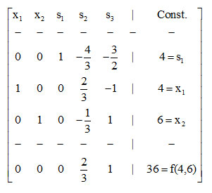
Working similarly with Example 1 it is straightforward to check that the last SIMPLEX matrix of the dual problem is the
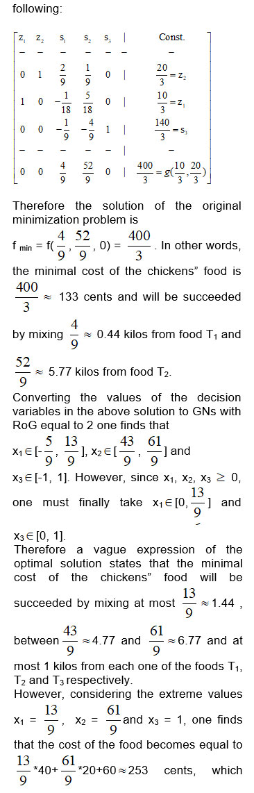
exceeds too much the minimal price of 133 cents. This means that the chosen RoG of the GNs is too large to provide a creditable vague expression of the problem’s solution. On the contrary, choosing for example the RoG to be equal
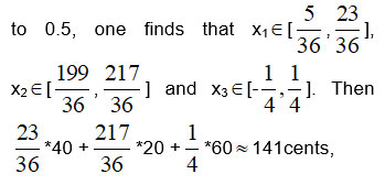
which is much closer to the minimal price of 133 cents. In general, the smaller is the chosen RoG of the GNs the more creditable is the vague expression of the problem’s solution.
Example 3: A cheese-making company produces three different types of cheeseT1, T2 and T3 by mixing cow-milk (C), sheep-milk (S) and milk powder (P). The required quantities in kilos from each kind of milk for producing a barrel of each of the three types of cheese are depicted, in form of GNs, in the following Table:
Table 1: Required quantities of milk 1
|
|
T1 |
T2 |
T3 |
|
C |
[1, 3] |
[5, 7] |
[0.5, 1.5] |
|
S |
[3, 5] |
[2, 4] |
[0.5, 1.5] |
|
P |
[0.8, 1.2] |
[0.3, 0.7] |
[0.2, 0.8] |
The cheese-maker’s profit from the sale of a barrel of cheese is 3 thousand euros for T1, 2 thousand euros for T3, whereas from the sale of a barrel of T2, the production of which becomes necessary for marketing reasons, there is a loss of 1 thousand euros.
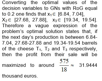
At the end of a certain day the stock of the cow-milk is high, so that at least 200 kilos of it must be used the next day, whereas the stock of the sheep-milk is 150 kilos. Further, there exists a stock of 100 kilos of expiring milk powder all of which must be spent the next day. Under the above conditions find with RoG equal to 0.2 which must be the next day’s production of cheese in order to maximize the profit from its sale.
Solution: Let x1, x2 and x3 be the barrels to be produced of cheese of the types T1, T2 and T3 respectively. Then the problem is mathematically formulated as follows:
Maximize
F = [3, 3]x1 - [1, 1]x2 + [2, 2]x3 subject to the constraints x1, x2 , x3 0 and
[1, 3]x1+ [5, 7]x2+ [0.5, 1.5]x3 >[200, 200],
[3, 5]x1+ [2, 4]x2+[1.5, 2.5]x3 > [150, 150]
[1.8,2.2]x1+[0.8,1.2]x2+[0.6,1.4]x3 => [100,100].
The whitenization of the GNs leads to the following LP maximization problem of general form 1.
Maximize f(x1, x2, x2) = 3x1 - x2 + 2x3 subject to the constraints x1,x2 ,x3> 0 and 2x1 + 6x2+ x3 >200
4x1 + 3x2 + 2x3 >150
2x1 + x2 + x3 = >100.
Adding the surplus variable s1 to the first inequality, the slack variable s2 to the second one and the artificial variables t1 and t2 to the first inequality and the last equation one turns all the special constraints to equations. Next, adding by members the two equations containing the artificial variables, one forms the problem’s first generalized SIMPLEX matrix as follows:
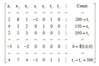
The rows of the artificial variables t1 and t2 are the, so called, anonymous rows of the above matrix. For the pivoting process, considering all the columns containing at least one positive number in the anonymous rows, we choose the one having the greatest positive number in the last row (of t1+t2), i.e. the column of x2. Then, since 200/6<150/3<100/1. the pivot element 6 lies in the first row. Therefore, applying the proper linear transformations among the rows of the matrix one forms the second generalized SIMPLEX matrix as follows:
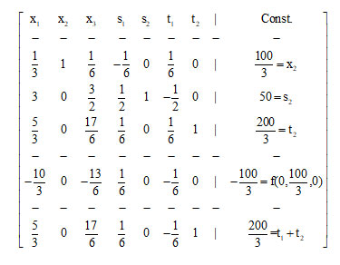
The pivot element 17/6 lies now in the intersection of the column of x3 and the row of t2 and the third generalized SIMPLEX matrix is the following:
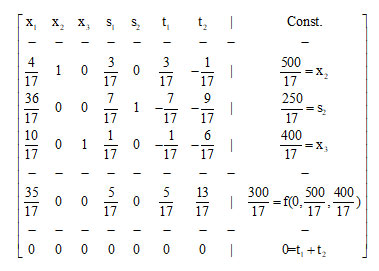
Therefore, omitting the last row and the columns of the artificial variables one obtains the problem’s first canonical SIMPLEX matrix.
Next, continuing the process in the standard way one finally reaches the optimal solution
Fmax = f(125/18,250/9,175/9)= 575/18.
Conclusion
A new technique was developed in this paper for solving Grey LP problems by the whitenization of the GNs involved in their statements and the solution of the ordinary LP problem obtained in this way with the standard theory. Real life examples were also presented to illustrate our method. In LP problems with fuzzy structure a vague expression of their solution is often preferable than the crisp one. This was attempted in the present work by converting the values of the decision variables in the optimal solution of the corresponding ordinary LP problem to GNs with the desired RoG. The smaller is the value of the chosen RoG, the more creditable the vague expression of the problem’s optimal solution.
An analogous method could be applied for solving fuzzy LP problems and systems of equations with grey or fuzzy data and this is the main target of our future research on the subject.
References
- Dantzig, G.B., Maximization of a linear function of variables subject to linear inequalities. Published in: T.C. Koopmans (Ed.): Activity Analysis of Production and Allocation. Wiley & Chapman - Hall, New York, London. 1951;339–347.
- Dantzig, G.B., Reminiscences about the origins of linear programming, Technical Report of Systems Optimization Laboratory 81-5, Department of Operations Research, Stanford University, CA. 1981.
- Wikipedia, Linear Programming, retrieved from https://en.wikipedia.org/wiki/Linear_programming on March 2018.
- Taha, H.A., Operations Research – An Introduction, Second Edition, Collier Macmillan, N.Y., London, 1967.
- Tanaka H., .Asai K., Fuzzy linear programming problems with fuzzy
numbers, Fuzzy Sets and Systems. 1984;13:1-10. - Verdegay, J.L., A dual approach to solve the fuzzy linear programming problem, Fuzzy Sets and Systems. 1984;14:131-141.
- Stephen Dinagar, D., Kamalanathan, S., Solving Linear Programming Problem Using New Ranking Procedures of Fuzzy Numbers, International Journal of Applications of Fuzzy Sets and Artificial Intelligence. 2017;281-292.
- Huang, G., Dan Moore, R., Grey linear programming, its solving approach, and its application, International Journal of Systems Science. 1993;24(1): 159-172.
- Seyed H., Razavi H., Akrami, H., Hashemi, S.S., A multi objective programming approach to solve grey linear programming, Grey Systems: Theory and Application. 2012;2(2):259-271.
- Voskoglou, M. Gr., Theodorou Y., Application of Grey Numbers to Assessment processes, International Journal of Applications of Fuzzy Sets and Artificial Intelligence. 2017;7:273-280.
- Liu, S. F. & Lin, Y. (Eds.), Advances in Grey System Research, Springer, Berlin – Heidelberg. 2010.

This work is licensed under a Creative Commons Attribution 4.0 International License.